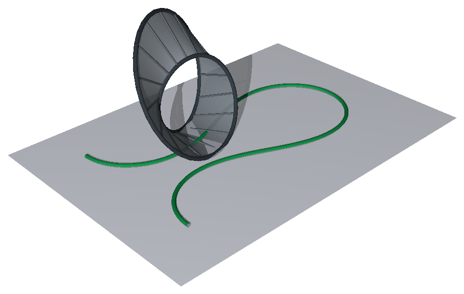
Take a coin and roll it along a table without letting it slip. The contact point traces a line on the table and a line on the coin, and the two lines have equal length — that is what “no slip” buys you. Now demand something stronger: as the coin rolls, it may not spin about the contact normal either. This is rolling without slip and without twist, a classical non-holonomic constraint: the velocity constraints cannot be integrated into position constraints, so where you end up genuinely depends on the path you rolled along.
Rolling has a clean home in geometric control theory, and rolling homogeneous spaces — spheres $S^n$, the rotation groups $SO_n$, Grassmannians — is by now well understood [Hüper & Silva Leite 2007; Jurdjevic 1997; Hüper, Kleinsteuber & Silva Leite 2008], because a transitive group action hands you a canonical parametrization for free. My 2015 master’s thesis — supervised by Prof. Dr. Knut Hüper, whom I thank for the guidance that made the whole thing possible — asked a question one step off that beaten path:
Can we roll the two most famous non-orientable surfaces — the Klein bottle and the Möbius band — on their tangent plane, and write down the motion explicitly?
It turns out you can, and the non-orientability is exactly what makes the setup interesting. This post is a showcase of the main results. The mathematics was worked out with SageMath, the open-source mathematics system; the three-dimensional figures below are then redrawn live in your browser from those same closed forms, so drag any of them to turn the surface around and look at it from another side.

What a rolling map actually is
Let $M\subset\mathbb{R}^n$ be a smooth submanifold, fix a start point $m_0\in M$, and let $V = m_0 + T_{m_0}M$ be the affine tangent plane there — the surface we roll on. A rigid motion of $\mathbb{R}^n$ is a curve in the special Euclidean group $SE_n = SO_n \ltimes \mathbb{R}^n$; write it as $h(t) = (R(t), s(t))$ acting by $p \mapsto R(t)p + s(t)$.
We call $h$ a rolling map of $M$ on $V$ if there is a rolling curve $\alpha:[0,\tau]\to M$ with $\alpha(0)=m_0$ such that, starting from $h(0)=(I_n,0)$:
- Rolling. The development $\alpha_{\mathrm{dev}}(t) := R(t)\alpha(t)+s(t)$ stays in the plane $V$, and $R(t)\,T_{\alpha(t)}M = T_{m_0}M$ (moving tangent spaces line up with the fixed one).
- No slip. $\dot R(t)\,\alpha(t) + \dot s(t) = 0$.
- No twist. With the angular velocity $\Omega := \dot R R^\top \in \mathfrak{so}_n$, $$\Omega\, T_{m_0}M \subseteq (T_{m_0}M)^\perp,\qquad \Omega\,(T_{m_0}M)^\perp \subseteq T_{m_0}M.$$
The development is the track the contact region leaves on the plane — the analogue of the coin’s line on the table. A theorem of Sharpe [Sharpe 1996] guarantees that a rolling curve or a development determines the whole rolling map uniquely; that bidirectionality is what later lets us run everything backwards.
One equation to rule them
The thesis’ organizing idea is to describe the manifold and every curve on it by an immersion, and read orthonormal tangent frames straight off it. If $v_1(t),\dots,v_k(t)$ is a moving orthonormal frame of $T_{\alpha(t)}M$ ($k=\dim M$), the rotational part always factors as
$$R(t) = P_0^\top\, S(t)\, P_0\, \hat R(t),$$where $\hat R$ transports the moving frame back to the start frame, $P_0\in O_n$ aligns the start frame with $e_1,\dots,e_k$, and $S(t)\in SO_n$ is block-diagonal, $S=\mathrm{diag}(K,L)$ with $K\in O_k$, $L\in O_l$. Writing $(\cdot)_{\mathrm{bd}}$ for the projection that kills the off-diagonal blocks, the no-twist conditions collapse to a single master ODE (the same $R = P_0^\top S P_0\hat R$ shape used for rolling Stiefel manifolds [Hüper, Kleinsteuber & Silva Leite 2008]):
$$\boxed{\;\dot S = -\,S\,\bigl(P_0\, \dot{\hat R}\, \hat R^\top\, P_0^\top\bigr)_{\mathrm{bd}}\;}$$together with the no-slip law $\dot s = -\dot R\,\alpha$. Everything below — both surfaces, forward and inverse — is a specialization of this one equation.
Why non-orientability is the whole point
The usual way to produce a submanifold is the regular value theorem: take $f^{-1}(c)$. But that construction only ever yields orientable manifolds. The Klein bottle and the Möbius band are not orientable, so that route is closed — which is precisely why the immersion approach is not a convenience here but a necessity.
Orientability is set up through nowhere-zero alternating $n$-forms [Amann & Escher 2008; Gallier 2015], and the thesis distills from it a reusable non-orientability criterion, applied to both surfaces: transport a tangent frame once around a generating loop $f(0)=f(1)$; if an odd number of frame vectors come back sign-flipped,
$$\lim_{t\to 1} t_k(t) = -\lim_{t\to 0} t_k(t)\quad\text{for an odd number of }k,$$the manifold is non-orientable. No global orientation exists to anchor a frame, so the moving frame $\hat R$ — and with it the rolling map — is the honest local object to compute with.
The Klein bottle in $S^3 \subset \mathbb{R}^4$
The Klein bottle does not embed in $\mathbb{R}^3$ [Spivak 1999], but Lawson’s minimal-surface parametrization [Lawson 1970] realizes it inside the 3-sphere $S^3\subset\mathbb{R}^4$:
$$k(x,y) = \begin{bmatrix} \sin x\cos y \\ \sin x\sin y \\ \cos x\cos\tfrac{y}{2} \\ \cos x\sin\tfrac{y}{2}\end{bmatrix}\in S^3\subset\mathbb{R}^4.$$The prettiest fact is that this immersion is a product of one-parameter subgroups, $k(x,y) = A(y)\,B(x)\,e_3$ with $A(y)=\exp(yX)$, $B(x)=\exp(xY)$ and fixed skew generators
$$X = \begin{bmatrix} 0&-1&0&0\\ 1&0&0&0\\ 0&0&0&-\tfrac12\\ 0&0&\tfrac12&0 \end{bmatrix},\qquad Y = \begin{bmatrix} 0&0&1&0\\ 0&0&0&1\\ -1&0&0&0\\ 0&-1&0&0 \end{bmatrix}.$$Look at $X$: it rotates by $y$ in the $(e_1,e_2)$-plane but by $y/2$ in $(e_3,e_4)$. That half-angle is the Klein-bottle twist made algebraic — go around once in $y$ and the last two coordinates have only turned halfway.
Seeing it in three dimensions
We can write $k$ down, but we cannot look at $S^3\subset\mathbb{R}^4$. To draw the surface we push it into ordinary space by stereographic projection. From the north pole $e_4$ this is the familiar map
$$\Pi_{e_4}:S^3\setminus\{e_4\}\to\mathbb{R}^3,\qquad x\mapsto \frac{1}{1-x_4}\begin{bmatrix}x_1\\ x_2\\ x_3\end{bmatrix},$$which slides each point along the ray from $e_4$ through it onto the equatorial hyperplane $\{x_4=0\}$, a diffeomorphism onto all of $\mathbb{R}^3$.
One condition decides whether the picture is any good: projection sends the pole itself off to infinity, so the pole must not lie on the surface you want to draw. The obvious choices fail here — both poles are on the bottle, since $e_4 = k(0,\pi)$ and $-e_4 = k(\pi,\pi)$. So we project instead from a point that is still on $S^3$ but off the surface,
$$\bar p = \Bigl[\,0,\ \tfrac{1}{\sqrt2},\ 0,\ \tfrac{1}{\sqrt2}\,\Bigr]^\top,$$by first rotating $\bar p$ onto the north pole with a fixed $C\in SO_4$ and then projecting — $\Pi_{\bar p} = \Pi_{e_4}\circ C$. This particular $\bar p$ earns its keep twice over: it dodges the surface, and it makes the projected bottle symmetric under $\mathrm{diag}(1,-1,-1)$, so the image is two congruent halves glued along their rims.

Taken by itself, one half is an open shell: it wraps around and passes back through a narrow neck into its own interior. Drawn alone — with the same coordinate net laid over it — that inner fold is easy to follow, the grid lines curving back through the neck as the surface does:

Because $\Pi_{\bar p}$ is a diffeomorphism it is injective, so it invents no crossings of its own: every self-intersection in the picture below is already present up in $S^3$. Those crossings are unavoidable — a closed non-orientable surface admits no embedding in three-space at all [Spivak 1999] — so what you see is the honest shadow of a surface that is perfectly smooth, merely passing through itself.

Feeding the frame factorization through the master ODE gives the kinematic equations for a rolling curve $\alpha(t)=k(x(t),y(t))$ (start $k(x_0,y_0)$, $R(0)=I_4$, $s(0)=0$):
$$\dot S = \dot y\,\frac{3\sin 2x}{2\sqrt{10-6\cos 2x}}\; S\, J,\qquad J=\begin{bmatrix} 0&-1&\\ 1&0&\\ &&0&\\ &&&0\end{bmatrix},$$$$\dot s = A(y_0)\tilde Q(x_0)^\top\, S\, \Bigl[\dot x,\; \tfrac{\dot y}{4}\sqrt{10-6\cos 2x},\; 0,\; 0\Bigr]^\top,\qquad R = A(y_0)\tilde Q(x_0)^\top\, S\, \tilde Q(x)A(y)^\top .$$Here $S=\mathrm{diag}(\tilde S, I_2)$ with $\tilde S\in SO_2$, and the recurring $\sqrt{10-6\cos 2x}$ is just $\lVert\partial k/\partial y\rVert$. Two features are worth pausing on:
- $\dot S$ depends only on $\dot y$. If $y$ is held constant, $S\equiv I_4$ and the rotation is entirely carried by the frame transport. So $k(t,c)$ rolls to a straight development — a geodesic.
- Because $S$ stabilizes $e_4$, the development collapses to $\alpha_{\mathrm{dev}}(t) = k_0 + s(t)$: a plane curve driven purely by the translational part.
Being planar, the development has a closed-form signed curvature. For the diagonal curve $k(t,t)$ it works out to
$$\kappa(t) = \frac{\sin 2t\,(63 - 9\cos 2t)} {\sqrt{13-3\cos 2t}^{\,3}\,\sqrt{5-3\cos 2t}},$$so the sign of the curvature is the sign of $\sin 2t$ — the development bends left, then right, alternating every $\pi/2$.
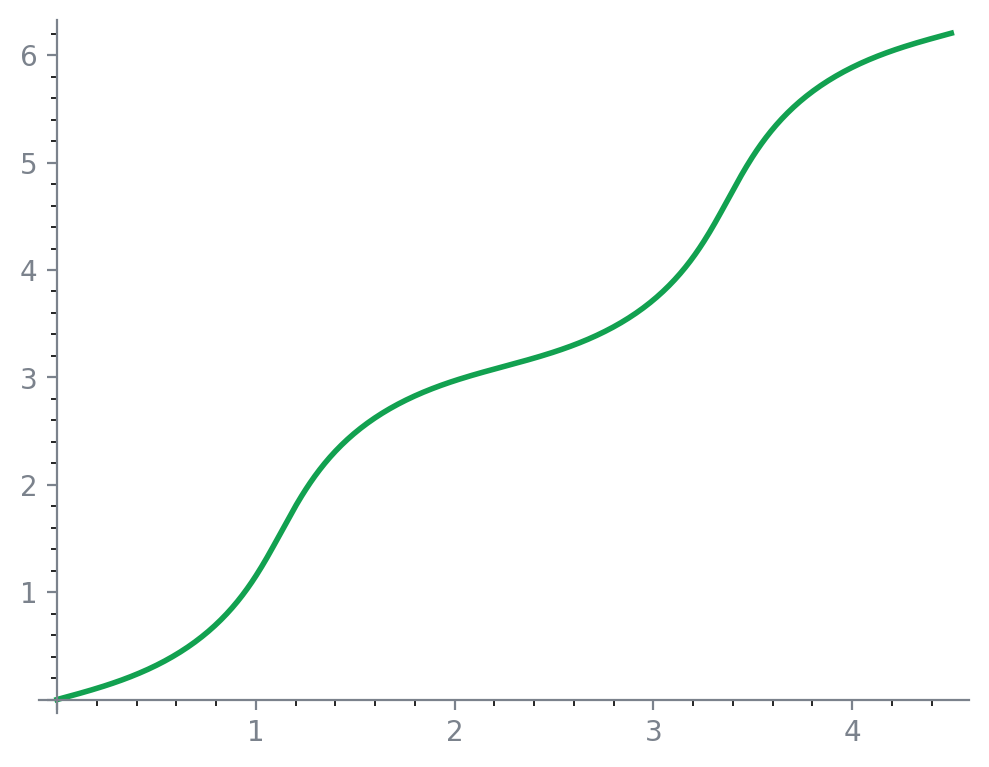 Development of $k(t,t)$: a wavy staircase in the plane.
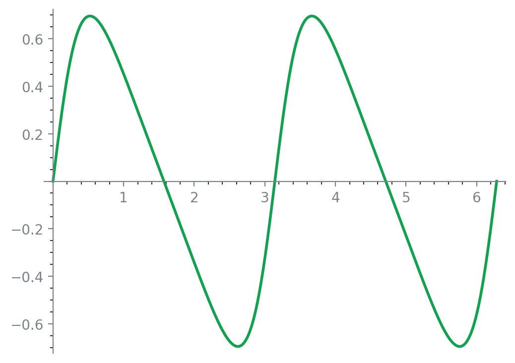 Its signed curvature $\kappa(t)$ — sign tracks $\sin 2t$, switching handedness
every $\pi/2$.
Its signed curvature $\kappa(t)$ — sign tracks $\sin 2t$, switching handedness
every $\pi/2$.
This is worth stating in general, because it decides which rolling problems have a closed form. A planar development is fixed, up to a rigid motion, by just two scalars: its speed and its signed curvature $\kappa$. Recovering the actual Cartesian coordinates is then one Fresnel/clothoid-type quadrature,
$$\mathrm{dev}(t) = \int \text{speed}\cdot[\cos\theta,\sin\theta]\,dt,\qquad \theta(t) = \int \kappa\,\text{speed}\,dt.$$So “is this case solvable in closed form?” splits into two independent questions — is the turning angle $\theta$ elementary, and is that final quadrature — and, as the examples below show, the answers can come out differently.
The Möbius band in $\mathbb{R}^3$
The Möbius band lives in ordinary space. Rescaling Forster’s parametrization [Forster 2012],
$$m(x,y) = \begin{bmatrix} \cos x\,\bigl(1 + \tfrac{y}{2}\cos\tfrac{x}{2}\bigr) \\ \sin x\,\bigl(1 + \tfrac{y}{2}\cos\tfrac{x}{2}\bigr) \\ \tfrac{y}{2}\sin\tfrac{x}{2}\end{bmatrix},\qquad y\in(-1,1),$$with $x$ the angle around the centre circle and $y$ the position across the width. The half-angle $x/2$ again encodes the twist: $m(x+2\pi,y)=m(x,-y)$.
With the orthonormal frame $P(x,y)=[t_1,t_2,n]^\top\in SO_3$ and the scalar
$$\delta(t) = \frac{y(3+2\cos x) + 8\cos\tfrac{x}{2}}{2\,\rho(x,y)},\qquad \rho = \sqrt{y^2(3+2\cos x) + 16y\cos\tfrac{x}{2} + 16},$$the master ODE specializes to the Möbius kinematic equations:
$$\dot S = -\dot x\,\delta\, S\, J_3,\quad J_3=\begin{bmatrix} 0&-1&0\\ 1&0&0\\ 0&0&0\end{bmatrix},\qquad R = P_0^\top S\, P(x,y),$$with $S=\mathrm{diag}(\tilde S,1)$. The mirror-image structure to the Klein bottle: here $\dot S$ depends only on $\dot x$, so moving purely across the width ($x$ constant) again gives $S\equiv I_3$ — and in fact $\alpha_{\mathrm{dev}}=\alpha$, the development coincides with the rolling curve.
The signature example is rolling the centre circle $m(t,0)$. Here the band genuinely rolls along the plane; the animation is worth more than the equation:

That development has an exact closed form — just not an elementary one, which makes it a nice test of the two-questions split above. It is the unit-speed curve of curvature $\kappa(t)=\cos(t/2)$, so its turning angle is elementary, $\theta(t)=2\sin(t/2)$; it is the Fresnel step that is not. Running it through Jacobi–Anger gives the Cartesian coordinates as an Anger–Weber / incomplete-Bessel series:
$$\mathrm{dev}_1(t) = J_0(2)\,t + \sum_{k\ge 1}\frac{2}{k}J_{2k}(2)\sin(kt),\qquad \mathrm{dev}_2(t) = 4\sum_{k\ge 0}\frac{J_{2k+1}(2)\,\bigl[1-\cos\bigl(\tfrac{(2k+1)t}{2}\bigr)\bigr]}{2k+1}.$$The Bessel values $J_m(2)$ decay super-exponentially, so about eight terms already reach machine precision — a reminder that non-elementary is not the same as no analytical solution.
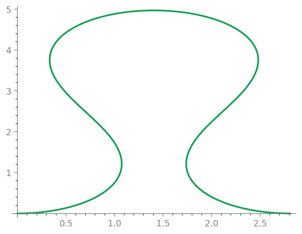 The exact Anger–Weber development of the centre-circle roll $m(t,0)$ — a closed,
symmetric plane curve computed from the Bessel series above.
The exact Anger–Weber development of the centre-circle roll $m(t,0)$ — a closed,
symmetric plane curve computed from the Bessel series above.
Rolling in reverse: the inverse problem and geodesics
Sharpe’s theorem says the development already determines the rolling map, so we can run the construction backwards: prescribe a plane curve $\alpha_{\mathrm{dev}}(t)=m_0+f(t)$ and solve for the rolling curve $\alpha$ that would produce it. Differentiating and using no-slip turns the top rows of the kinematic equations into an ODE for $(x(t),y(t))$ coupled to the same $S$-ODE.
The payoff is a clean characterization of geodesics:
A rolling curve is a geodesic iff its development is a straight line.
So feeding a straight $f$ into the inverse equations manufactures geodesics.
For the Klein bottle this can be pushed all the way to a closed form. Its induced metric under the Lawson immersion is diagonal and, remarkably, independent of $y$: $g = dx^2 + G(x)\,dy^2$ with $G(x) = 1 - \tfrac34\cos^2 x$. That makes $y$ cyclic, so a geodesic carries two first integrals (Clairaut + energy) and reduces to an elliptic quadrature:
$$t(x) = \int_{x_0}^{x}\frac{dx'}{\sqrt{E - L^2/G(x')}},\qquad y(x) = y_0 + \int_{x_0}^{x}\frac{L/G(x')}{\sqrt{E - L^2/G(x')}}\,dx'.$$
The Möbius band is less obliging — as we will see, its metric denies exactly this shortcut — but the inverse construction still runs numerically:

There is a catch unique to the Möbius band, and it is geometrically honest: the inverse ODE can drive $y(t)$ out of $(-1,1)$, i.e. off the edge of the band. When that happens the rolling map only exists up to the first exit time. So not every development corresponds to a rolling curve — the band’s finite width alone already kills global controllability [cf. Krakowski & Silva Leite 2012]. (Local controllability remains open, and as far as I can tell still is; see the outlook.)
Where this could go
Two kinds of open problem remain, one analytical and one geometric.
Which cases are truly closed? The closed forms above are proven; the negative side — that the cases still left numerical (the $s$-integral that completes $k(t,t)$, the angle quadrature of a fast winding like $k(t,e^t)$, the Möbius geodesics) have no elementary form — is so far only heuristic. A CAS failing to integrate is evidence, not a proof, and two different machineries would settle it. For the antiderivative cases the rigorous criterion is Liouville’s theorem with the Risch algorithm as decision procedure — but Risch is only complete for purely transcendental integrands, and these carry algebraic radicals like $\sqrt{10-6\cos 2t}$, so every CAS is only partial and a by-hand argument is needed. The geodesic/ODE cases are a different problem — integrability by quadratures, not antiderivatives, so Liouville/Risch do not apply. The Klein bottle is solvable precisely because its $y$-independent metric hands you a linear first integral; the Möbius metric $g_{xx}(x,y)$ depends on both coordinates, so one would need a Killing-tensor search for a quadratic first integral, or a non-integrability proof via differential Galois theory (Morales–Ramis).
And the geometry. The niche is still surprisingly empty: as of 2026 I’ve found no published work that rolls a non-orientable surface and works out its kinematics or controllability explicitly. The concrete openings — a homogeneous-space re-derivation (both surfaces are homogeneous, by Mostow [Mostow 1950]), and the local controllability of the Möbius-band roll — are still there for the taking.
References
- H. Amann, J. Escher. Analysis II / III. Birkhäuser, 2008.
- O. Forster. Analysis 3. Vieweg+Teubner, 2012.
- J. Gallier. Notes on Differential Geometry and Lie Groups. 2015.
- K. Hüper, M. Kleinsteuber, F. Silva Leite. Rolling Stiefel manifolds. International Journal of Systems Science 30(9) (2008) 881–887.
- K. Hüper, F. Silva Leite. On the geometry of rolling and interpolation curves on $S^n$, $SO_n$, and Grassmann manifolds. Journal of Dynamical and Control Systems 13(4) (2007) 467–502.
- V. Jurdjevic. Geometric Control Theory. Cambridge University Press, 1997.
- K. A. Krakowski, F. Silva Leite. Why controllability of rolling motions may fail. CONTROLO 2012, 197–203.
- H. B. Lawson Jr. Complete minimal surfaces in $S^3$. Annals of Mathematics 92(2) (1970) 335–374.
- G. D. Mostow. The extensibility of local Lie groups of transformations and groups on surfaces. Annals of Mathematics 52(3) (1950) 606–636.
- R. W. Sharpe. Differential Geometry. Springer, 1996.
- M. Spivak. A Comprehensive Introduction to Differential Geometry, Vol. 1. Publish or Perish, 1999.